Quickstart

Hénon-Heiles Example

We consider the system of Hénon-Heiles satisfied by $u(t)=(u_1, u_2, u_3, u_4)(t)$.

\[\frac{d u }{dt} = \frac{1}{\varepsilon} Au + f(u), \;\;\; u(t_{start})=u_{inn}\in\mathbb{R}^4,\]

where $A$ and $f$ are selected as follows

\[A= \left( \begin{array}{cccc} 0 & 0 & 1 & 0 \\ 0 & 0 & 0 & 0 \\ -1 & 0 & 0 & 0 \\ 0 & 0 & 0 & 0 \end{array} \right) \;\;\;\; \text{ and } \;\;\;\; f(u) = \left( \begin{array}{cccc} 0 \\ u_4\\ -2 u_1 u_2\\ -u_2-u_1^2+u_2^2 \end{array} \right).\]

one chooses for example, $\varepsilon=0.001$ and $u_{in} = (0.12, 0.12, 0.12, 0.12)$

Input parameters

The input arguments use the same format as the ODE package.

Thus, first of all, we must define the arguments necessary to construct the problem (1), namely

the $f$ function (in the form Julia)
the initial condition $u_{in}$.
the initial time $t_{start}$ and final time $t_{end}$.
the second parameter of the
the $A$ matrix
$\varepsilon \in ]0, 1]$

using HOODESolver, Plots

epsilon= 0.0001

A = [ 0 0 1 0 ;
      0 0 0 0 ;
     -1 0 0 0 ;
      0 0 0 0 ]

f1 = LinearHOODEOperator( epsilon, A)

f2 = (u,p,t) ->  [ 0, u[4], 2*u[1]*u[2], -u[2] - u[1]^2 + u[2]^2 ]

tspan = (0.0, 3.0)

u0 = [0.55, 0.12, 0.03, 0.89]

prob = SplitODEProblem(f1, f2, u0, tspan);

From the prob problem, we can now switch to its numerical resolution.

To do this, the numerical parameters are defined

the number of time slots $N_t$ which defines the time step $\Delta t = \frac{t_{\text{end}}-t_{start}}{N_t}$ but you can set the value of time step dt in the solve call.
the $r$ order of the method
the number of $N_\tau$ points in the $\tau$ direction...
the order of preparation $q$ of the initial condition

The default settings are : $N_t=100$, $r=4$, $N_\tau=32$ and $q=r+2=6$ To solve the problem with the default parameters, just call the solve command with the problem already defined as parameter

sol = solve(prob, HOODEAB(), dt=0.1);

solve function prob=HOODEProblem{Float64}(HOODESolver.HOODEFunction{false, 3}(Main.var"#1#2"()), [0.55, 0.12, 0.03, 0.89], (0.0, 3.0), missing, [0 0 1 0; 0 0 0 0; -1 0 0 0; 0 0 0 0], 0.0001, missing),
 nb_tau=32, order=4, order_prep=6, dense=true,
 nb_t=30, getprecision=true, verbose=100

 30/30

 35/35

Which is equivalent to HOODEAB( order=4, nb_tau=32 )

Exhaustive definition of the parameters

prob : problem defined by SplitODEProblem
nb_tau=32 : $N_{\tau}$
order=4 : order $r$ of the method
order_prep=order+2 : order of preparation of initial data
dense=true : indicates whether or not to keep the data from the fourier transform, if dense=false, processing is faster but interpolation can no longer be done.
nb_t=100 : $N_t$
getprecision=dense : indicates whether the accuracy is calculated, the method used to calculate the accuracy multiplies the processing time by 2.
verbose=100 : trace level, if verbose=0 then nothing is displayed.
par_u0 : If we have to make several calls to solve with the same initial data and in the same order, we can pass in parameter the already calculated data.
p_coef : table with the coefficients of the Adams-Bashforth method. This array can be used to optimize several calls with the same parameters.

Exit arguments

As an output, a structure of type ODESolution from DifferentialEquations.jl. This structure can be seen as a function of t, it can also be seen as an array. Example:

julia> sol.probODEProblem with uType Vector{Float64} and tType Float64. In-place: false
timespan: (0.0, 3.0)
u0: 4-element Vector{Float64}:
 0.55
 0.12
 0.03
 0.89
julia> sol.algHOODESolver.HOODETwoScalesAB()
julia> t=2.5414515472.541451547
julia> sol(t)4-element Vector{Float64}:
 -0.5364409362202105
  1.5936478974018409
 -0.1244826793694423
  0.718925898254452
julia> sol[end]4-element Vector{Float64}:
  0.36354863065271914
  2.0384405589059846
 -0.4134978102269046
  1.3093799931994603
julia> sol(3.0)4-element Vector{Float64}:
  0.3635486306933823
  2.038440559226788
 -0.41349781031083227
  1.3093799933836259

To view the result, you can also use Plot, for example

plot(sol)

Linear non-homogeneous case

The following non-homogeneous linear system is considered to be satisfied by $u(t)=(u_1, u_2, u_3, u_4)(t)$

\[\frac{d u }{dt} = \frac{1}{\varepsilon} Au + f(t, u), \;\;\; u(0)=u_in\in\mathbb{R}^4,\]

where $A$ and $f$ are selected as follows

\[A= \left( \begin{array}{cccc} 0 & 0 & 1 & 0 \\ 0 & 0 & 0 & 0 \\ -1 & 0 & 0 & 0 \\ 0 & 0 & 0 & 0 \end{array} \right) \;\;\; \text{ and } \;\;\; f(t, u) = Bu +\alpha t +\beta \;\; \text{ with } \;\; B\in {\mathcal M}_{4, 4}(\mathbb{R}), \alpha, \beta \in \mathbb{R}^4,\]

$B, \alpha, \beta$ are chosen randomly.

We wish to obtain a high precision, so we will use BigFloat real numbers, they are encoded on 256 bits by default which gives a precision bound of about $2^{-256}. \approx 10^{-77}$. At the end, we compare a calculated result with an exact result. For this, you must use the dedicated HOODEProblem type:

using HOODESolver
using Plots
using Random

rng = MersenneTwister(1111)

A=[0 0 1 0 ; 0 0 0 0 ; -1 0 0 0 ; 0 0 0 0]
B = 2rand(rng, BigFloat, 4, 4) - ones(BigFloat, 4, 4)
alpha = 2rand(rng, BigFloat, 4) - ones(BigFloat, 4)
beta = 2rand(rng, BigFloat, 4) - ones(BigFloat, 4)
u0 = [big"0.5", big"-0.123", big"0.8", big"0.7"]
t_start=big"0.0"
t_end=big"1.0"
epsilon=big"0.017"

fct = (u,p,t)-> B*u + t*p[1] +p[2]

prob = HOODEProblem(fct, u0, (t_start,t_end), (alpha, beta), A, epsilon, B)

sol = solve(prob, nb_t=10000, order=8)
sol.absprec

7.505703231386974e-36

t=big"0.9756534187771"
sol(t)-getexactsol(sol.par_u0.parphi, u0, t)

4-element Vector{BigFloat}:
 -6.642791236756757511842356739364490481272378844877623661270313373986460667182805e-38
 -1.32710740831924512493061931801550544383767245077494551171855339990396286340094e-36
  1.238667480541656513250587460280152711356707094227379112388964758165354977619083e-36
 -1.15516259158393487305792694336447883915887578982651641650090295550219560023191e-35

plot(sol.t,sol.u_tr)

Calculation of the exact solution

This involves calculating the exact solution $u(t)$ of the following equation at the instant $t$

\[\frac{d u }{dt} = \frac{1}{\varepsilon} Au + Bu +\alpha t +\beta, \;\;\; u(t_{start})=u_{in}\in\mathbb{R}^4\text{, } A \text{ and }B \text{ are defined above }\]

Let

\[\begin{aligned} M &= \frac{1}{\varepsilon} A + B\\ C &= e^{-t_{start} M}u_{in} +M^{-1} e^{-t_{start} M} (t_{start}\alpha+\beta)+ M^{-2} e^{-t_{start} M} \alpha\\ C_t &= -M^{-1} e^{-t M} (t\alpha+\beta)-M^{-2} e^{-t M} \alpha\\ u(t) &= e^{t M} ( C + C_t) \end{aligned}\]

Which, translated into Julia language, gives the code of the function getexactsol :

function getexactsol(par::PreparePhi, u0, t)
    @assert !ismissing(par.matrix_B) "The debug matrix is not defined"
    sparse_A = par.sparse_Ap[1:(end-1),1:(end-1)]
    m = (1/par.epsilon)*sparse_A+par.matrix_B
    t_start = par.t_0
    if ismissing(par.paramfct)
        return exp((t-t0)*m)*u0
    end
    a, b = par.paramfct
    mm1 = m^(-1)
    mm2 = mm1^2
    e_t0 = exp(-t_start*m)
    C = e_t0*u0 + mm1*e_t0*(t_start*a+b)+mm2*e_t0*a
    e_inv = exp(-t*m)
    e = exp(t*m)
    C_t = -mm1*e_inv*(t*a+b)-mm2*e_inv*a
    return e*C+e*C_t
end

Accuracy of the result according to the time interval

Linear problem

From a problem of the previous type, as long as we can calculate the exact solution, it is possible to know exactly what the error is. The initialization data being

using HOODESolver

A = [0 0 1 0 ; 0 0 0 0 ; -1 0 0 0 ; 0 0 0 0]

u0 = BigFloat.([-34//100, 78//100, 67//100, -56//10])

B = BigFloat.([12//100 -78//100 91//100 34//100
    -45//100 56//100 3//100 54//100
    -67//100 09//100 18//100 89//100
    -91//100 -56//100 11//100 -56//100])

alpha =  BigFloat.([12//100, -98//100, 45//100, 26//100])

beta =  BigFloat.([-4//100, 48//100, 23//100, -87//100])

epsilon = 0.015

t_end = big"1.0"

fct = (u,p,t)-> B*u + t*p[1] +p[2]

prob = HOODEProblem(fct,u0, (big"0.0",t_end), (alpha, beta), A, epsilon, B)

Note that the floats are coded on 512 bits.
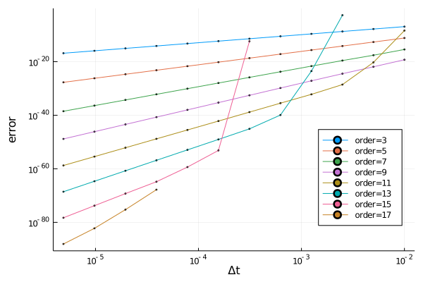
By varying $\Delta t$ from $10^{-2}$ to $5.10^{-6}$ (i.e. nb_t from 100 to 204800) on a logarithmic scale, for odd orders from 3 to 17 we get these errors

u0=BigFloat.([90, -44, 83, 13]//100)
t_end = big"1.0"
epsilon=big"0.0017"
fct = u -> [0, u[4], -2u[1]*u[2], -u[2]-u[1]^2+u[2]^2]
A = [0 0 1 0; 0 0 0 0;-1 0 0 0; 0 0 0 0]
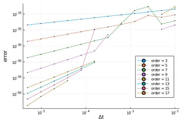
prob = HOODEProblem(fct, u0, (big"0.0",t_end), missing, A, epsilon)

The float are coded on 512 bits.

Precision of the result with ε = 0.0017

Now with the same initial data, order being setted to 6, and $\varepsilon = 0.19, 0.019, \ldots, 1.9\times 10^{-8}$.
Here floats are coded on 256 bits.