Numpy#
What provide Numpy to Python ?#
ndarraymulti-dimensional array objectderived objects such as masked arrays and matrices
ufuncfast array mathematical operations.Offers some Matlab-ish capabilities within Python
Initially developed by Travis Oliphant.
Numpy 1.0 released October, 2006.
The SciPy.org website is very helpful.
NumPy fully supports an object-oriented approach.
Routines for fast operations on arrays.#
shape manipulation
sorting
I/O
FFT
basic linear algebra
basic statistical operations
random simulation
statistics
and much more…
Getting Started with NumPy#
It is handy to import everything from NumPy into a Python console:
from numpy import *
But it is easier to read and debug if you use explicit imports.
import numpy as np
import scipy as sp
import matplotlib.pyplot as plt
import numpy as np
print(np.__version__)
2.2.6
Why Arrays ?#
Python lists are slow to process and use a lot of memory.
For tables, matrices, or volumetric data, you need lists of lists of lists… which becomes messy to program.
from random import random
from operator import truediv
l1 = [random() for i in range(1000)]
l2 = [random() for i in range(1000)]
%timeit s = sum(map(truediv,l1,l2))
23.2 μs ± 50.8 ns per loop (mean ± std. dev. of 7 runs, 10,000 loops each)
a1 = np.array(l1)
a2 = np.array(l2)
%timeit s = np.sum(a1/a2)
3.61 μs ± 17.4 ns per loop (mean ± std. dev. of 7 runs, 100,000 loops each)
Numpy Arrays: The ndarray class.#
There are important differences between NumPy arrays and Python lists:
NumPy arrays have a fixed size at creation.
NumPy arrays elements are all required to be of the same data type.
NumPy arrays operations are performed in compiled code for performance.
Most of today’s scientific/mathematical Python-based software use NumPy arrays.
NumPy gives us the code simplicity of Python, but the operation is speedily executed by pre-compiled C code.
a = np.array([0,1,2,3])  #  list
b = np.array((4,5,6,7))  #  tuple
c = np.matrix('8 9 0 1') #  string (matlab syntax)
print(a,b,c)
[0 1 2 3] [4 5 6 7] [[8 9 0 1]]
Element wise operations are the “default mode”#
a*b,a+b
(array([ 0, 5, 12, 21]), array([ 4, 6, 8, 10]))
5*a, 5+a
(array([ 0, 5, 10, 15]), array([5, 6, 7, 8]))
a @ b, np.dot(a,b) # Matrix multiplication
(np.int64(38), np.int64(38))
NumPy Arrays Properties#
a = np.array([1,2,3,4,5]) # Simple array creation
type(a) # Checking the type
numpy.ndarray
a.dtype # Print numeric type of elements
dtype('int64')
a.itemsize # Print Bytes per element
8
a.shape # returns a tuple listing the length along each dimension
(5,)
np.size(a), a.size # returns the entire number of elements.
(5, 5)
a.ndim # Number of dimensions
1
a.nbytes # Memory used
40
** Always use
shapeorsizefor numpy arrays instead oflen**lengives same information only for 1d array.
Functions to allocate arrays#
x = np.zeros((2,),dtype=('i4,f4,a10'))
x
/tmp/ipykernel_7745/3891786444.py:1: DeprecationWarning: Data type alias 'a' was deprecated in NumPy 2.0. Use the 'S' alias instead.
  x = np.zeros((2,),dtype=('i4,f4,a10'))
array([(0, 0., b''), (0, 0., b'')],
      dtype=[('f0', '<i4'), ('f1', '<f4'), ('f2', 'S10')])
empty, empty_like, ones, ones_like, zeros, zeros_like, full, full_like
Setting Array Elements Values#
a = np.array([1,2,3,4,5])
print(a.dtype)
int64
a[0] = 10 # Change first item value
a, a.dtype
(array([10, 2, 3, 4, 5]), dtype('int64'))
a.fill(0) # slighty faster than a[:] = 0
a
array([0, 0, 0, 0, 0])
Setting Array Elements Types#
b = np.array([1,2,3,4,5.0]) # Last item is a float
b, b.dtype
(array([1., 2., 3., 4., 5.]), dtype('float64'))
a.fill(3.0)  # assigning a float into a int array
a[1] = 1.5   # truncates the decimal part
print(a.dtype, a)
int64 [3 1 3 3 3]
a.astype('float64') # returns a new array containing doubles
array([3., 1., 3., 3., 3.])
np.asfarray([1,2,3,4]) # Return an array converted to a float type
---------------------------------------------------------------------------
AttributeError                            Traceback (most recent call last)
Cell In[25], line 1
----> 1 np.asfarray([1,2,3,4]) # Return an array converted to a float type

File ~/miniconda3/envs/runenv/lib/python3.13/site-packages/numpy/__init__.py:400, in __getattr__(attr)
    397     raise AttributeError(__former_attrs__[attr], name=None)
    399 if attr in __expired_attributes__:
--> 400     raise AttributeError(
    401         f"`np.{attr}` was removed in the NumPy 2.0 release. "
    402         f"{__expired_attributes__[attr]}",
    403         name=None
    404     )
    406 if attr == "chararray":
    407     warnings.warn(
    408         "`np.chararray` is deprecated and will be removed from "
    409         "the main namespace in the future. Use an array with a string "
    410         "or bytes dtype instead.", DeprecationWarning, stacklevel=2)

AttributeError: `np.asfarray` was removed in the NumPy 2.0 release. Use `np.asarray` with a proper dtype instead.
Slicing x[lower:upper:step]#
Extracts a portion of a sequence by specifying a lower and upper bound.
The lower-bound element is included, but the upper-bound element is not included.
The default step value is 1 and can be negative.
a = np.array([10,11,12,13,14])
a[:2], a[-5:-3], a[0:2], a[-2:] # negative indices work
(array([10, 11]), array([10, 11]), array([10, 11]), array([13, 14]))
a[::2], a[::-1]
(array([10, 12, 14]), array([14, 13, 12, 11, 10]))
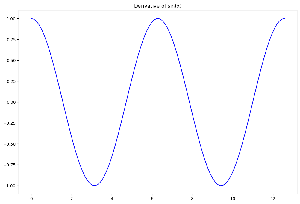
Exercise:#
Compute derivative of \(f(x) = \sin(x)\) with finite difference method. $\( \frac{\partial f}{\partial x} \sim \frac{f(x+dx)-f(x)}{dx} \)$
derivatives values are centered in-between sample points.
x, dx = np.linspace(0,4*np.pi,100, retstep=True)
y = np.sin(x)
%matplotlib inline
import matplotlib.pyplot as plt
plt.rcParams['figure.figsize'] = [12.,8.] # Increase plot size
plt.plot(x, np.cos(x),'b')
plt.title(r"$\rm{Derivative\ of}\ \sin(x)$");
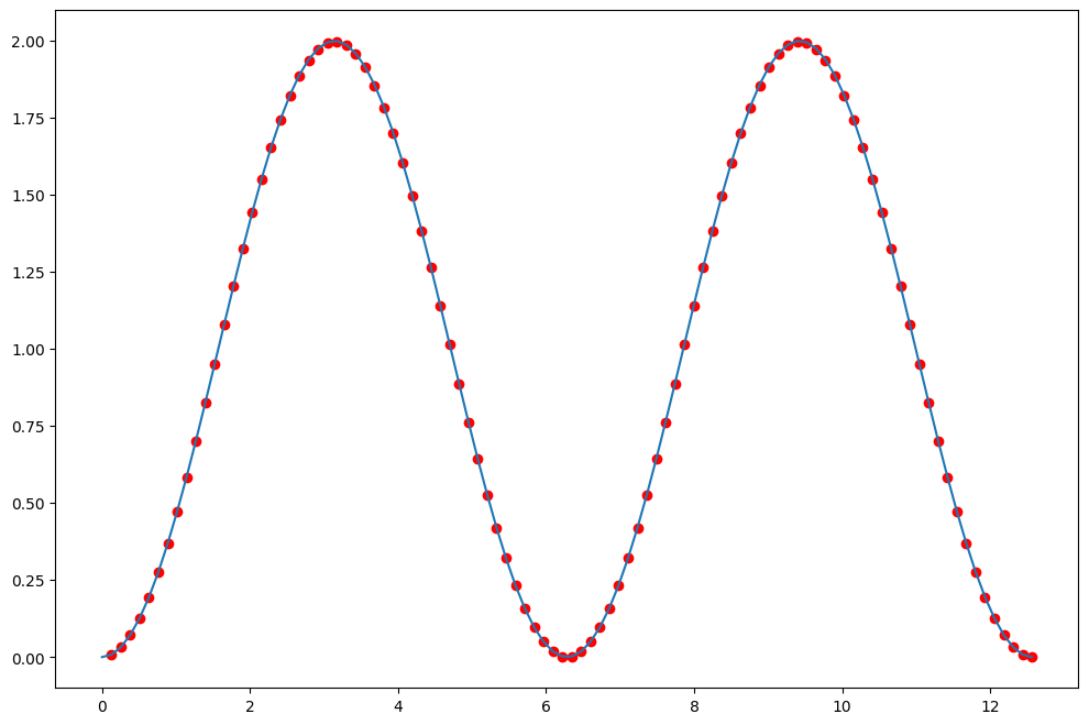
# Compute integral of x numerically
avg_height = 0.5*(y[1:]+y[:-1])
int_sin = np.cumsum(dx*avg_height)
plt.plot(x[1:], int_sin, 'ro', x, np.cos(0)-np.cos(x));
Multidimensional array#
a = np.arange(4*3).reshape(4,3) # NumPy array
l = [[0,1,2],[3,4,5],[6,7,8],[9,10,11]] # Python List
print(a)
print(l)
[[ 0  1  2]
 [ 3  4  5]
 [ 6  7  8]
 [ 9 10 11]]
[[0, 1, 2], [3, 4, 5], [6, 7, 8], [9, 10, 11]]
l[-1][-1] # Access to last item
11
print(a[-1,-1])  # Indexing syntax is different with NumPy array
print(a[0,0])    # returns the first item
print(a[1,:])    # returns the second line
11
0
[3 4 5]
print(a[1]) # second line with 2d array
print(a[:,-1])  # last column
[3 4 5]
[ 2  5  8 11]
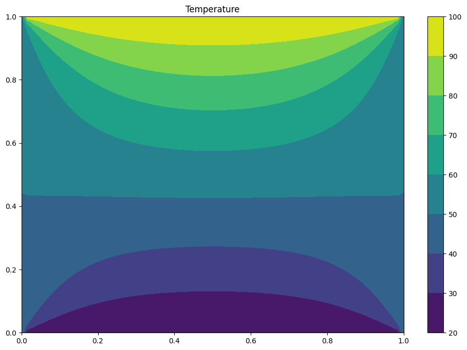
Exercise#
We compute numerically the Laplace Equation Solution using Finite Difference Method
Replace the computation of the discrete form of Laplace equation with numpy arrays $\( \Delta T_{i,j} = ( T_{i+1,j} + T_{i-1,j} + T_{i,j+1} + T_{i,j-1} - 4 T_{i,j}) \)$
The function numpy.allclose can help you to compute the residual.
%%time
# Boundary conditions
Tnorth, Tsouth, Twest, Teast = 100, 20, 50, 50

# Set meshgrid
n, l = 64, 1.0
X, Y = np.meshgrid(np.linspace(0,l,n), np.linspace(0,l,n))
T = np.zeros((n,n))

# Set Boundary condition
T[-1, :] = Tnorth
T[0, :]   = Tsouth
T[:, -1] = Teast
T[:, 0]   = Twest

T_old = np.copy(T)

residual = 1.0
istep = 0
while residual > 1e-5 :
    istep += 1
    print ((istep, residual), end="\r")
    residual = 0.0
    for i in range(1, n-1):
        for j in range(1, n-1):
            T_old[i,j] = T[i,j]
            T[i, j] = 0.25 * (T[i+1,j] + T[i-1,j] + T[i,j+1] + T[i,j-1])

    residual = max(residual,np.max(np.abs((T_old-T)/T)))


print()
print("iterations = ",istep)
plt.title("Temperature")
plt.contourf(X, Y, T)
plt.colorbar();
(2457, 1.0022293826789268e-05)
iterations =  2457
CPU times: user 18.9 s, sys: 84.1 ms, total: 19 s
Wall time: 19 s
<matplotlib.colorbar.Colorbar at 0x114e1e3b0>
Arrays to ASCII files#
x = y = z = np.arange(0.0,5.0,1.0)
np.savetxt('test.out', (x,y,z), delimiter=',')   # X is an array
%cat test.out
0.000000000000000000e+00,1.000000000000000000e+00,2.000000000000000000e+00,3.000000000000000000e+00,4.000000000000000000e+00
0.000000000000000000e+00,1.000000000000000000e+00,2.000000000000000000e+00,3.000000000000000000e+00,4.000000000000000000e+00
0.000000000000000000e+00,1.000000000000000000e+00,2.000000000000000000e+00,3.000000000000000000e+00,4.000000000000000000e+00
np.savetxt('test.out', (x,y,z), fmt='%1.4e')   # use exponential notation
%cat test.out
0.0000e+00 1.0000e+00 2.0000e+00 3.0000e+00 4.0000e+00
0.0000e+00 1.0000e+00 2.0000e+00 3.0000e+00 4.0000e+00
0.0000e+00 1.0000e+00 2.0000e+00 3.0000e+00 4.0000e+00
Arrays from ASCII files#
np.loadtxt('test.out')
array([[0., 1., 2., 3., 4.],
       [0., 1., 2., 3., 4.],
       [0., 1., 2., 3., 4.]])
save: Save an array to a binary file in NumPy .npy format
savez : Save several arrays into an uncompressed .npz archive
savez_compressed: Save several arrays into a compressed .npz archive
load: Load arrays or pickled objects from .npy, .npz or pickled files.
H5py#
Pythonic interface to the HDF5 binary data format. h5py user manual
import h5py as h5

with h5.File('test.h5','w') as f:
    f['x'] = x
    f['y'] = y
    f['z'] = z
with h5.File('test.h5','r') as f:
    for field in f.keys():
        print(field+':',np.array(f.get("x")))
x: [0. 1. 2. 3. 4.]
y: [0. 1. 2. 3. 4.]
z: [0. 1. 2. 3. 4.]
Slices Are References#
Slices are references to memory in the original array.
Changing values in a slice also changes the original array.
a = np.arange(10)
b = a[3:6]
b  # `b` is a view of array `a` and `a` is called base of `b`
array([3, 4, 5])
b[0] = -1
a  # you change a view the base is changed.
array([ 0, 1, 2, -1, 4, 5, 6, 7, 8, 9])
Numpy does not copy if it is not necessary to save memory.
c = a[7:8].copy() # Explicit copy of the array slice
c[0] = -1
a
array([ 0, 1, 2, -1, 4, 5, 6, 7, 8, 9])
Fancy Indexing#
a = np.fromfunction(lambda i, j: (i+1)*10+j, (4, 5), dtype=int)
a
array([[10, 11, 12, 13, 14],
       [20, 21, 22, 23, 24],
       [30, 31, 32, 33, 34],
       [40, 41, 42, 43, 44]])
np.random.shuffle(a.flat) # shuffle modify only the first axis
a
array([[31, 10, 42, 11, 21],
       [24, 22, 32, 14, 13],
       [44, 34, 33, 20, 41],
       [40, 30, 23, 43, 12]])
locations = a % 3 == 0 # locations can be used as a mask
a[locations] = 0 #set to 0 only the values that are divisible by 3
a
array([[31, 10,  0, 11,  0],
       [ 0, 22, 32, 14, 13],
       [44, 34,  0, 20, 41],
       [40,  0, 23, 43,  0]])
a += a == 0
a
array([[31, 10,  1, 11,  1],
       [ 1, 22, 32, 14, 13],
       [44, 34,  1, 20, 41],
       [40,  1, 23, 43,  1]])
numpy.take#
a[1:3,2:5]
array([[32, 14, 13],
       [ 1, 20, 41]])
np.take(a,[[6,7],[10,11]]) # Use flatten array indices
array([[22, 32],
       [44, 34]])
Changing array shape#
grid = np.indices((2,3)) # Return an array representing the indices of a grid.
grid[0]
array([[0, 0, 0],
       [1, 1, 1]])
grid[1]
array([[0, 1, 2],
       [0, 1, 2]])
grid.flat[:] # Return a view of grid array
array([0, 0, 0, 1, 1, 1, 0, 1, 2, 0, 1, 2])
grid.flatten() # Return a copy
array([0, 0, 0, 1, 1, 1, 0, 1, 2, 0, 1, 2])
np.ravel(grid, order='C') # A copy is made only if needed.
array([0, 0, 0, 1, 1, 1, 0, 1, 2, 0, 1, 2])
Sorting#
a=np.array([5,3,6,1,6,7,9,0,8])
np.sort(a) # Return a copy
array([0, 1, 3, 5, 6, 6, 7, 8, 9])
a
array([5, 3, 6, 1, 6, 7, 9, 0, 8])
a.sort() # Change the array inplace
a
array([0, 1, 3, 5, 6, 6, 7, 8, 9])
Transpose-like operations#
a = np.array([5,3,6,1,6,7,9,0,8])
b = a
b.shape = (3,3) # b is a reference so a will be changed
a
array([[5, 3, 6],
       [1, 6, 7],
       [9, 0, 8]])
c = a.T # Return a view so a is not changed
np.may_share_memory(a,c)
True
c[0,0] = -1 # c is stored in same memory so change c you change a
a
array([[-1,  3,  6],
       [ 1,  6,  7],
       [ 9,  0,  8]])
c # is a transposed view of a
array([[-1,  1,  9],
       [ 3,  6,  0],
       [ 6,  7,  8]])
b # b is a reference to a
array([[-1,  3,  6],
       [ 1,  6,  7],
       [ 9,  0,  8]])
c.base # When the array is not a view `base` return None
array([[-1,  3,  6],
       [ 1,  6,  7],
       [ 9,  0,  8]])
Methods Attached to NumPy Arrays#
a = np.arange(20).reshape(4,5)
np.random.shuffle(a.flat)
a
array([[ 0, 13,  1, 19, 11],
       [14,  3,  6,  4,  8],
       [15,  5, 12, 18,  7],
       [10,  9, 16,  2, 17]])
a -= a.mean()
a /= a.std() # Standardize the matrix

a.std(), a.mean()
(1.0, -1.1102230246251566e-17)
np.set_printoptions(precision=4)
print(a)
[[-1.6475  0.607  -1.4741  1.6475  0.2601]
 [ 0.7804 -1.1272 -0.607  -0.9538 -0.2601]
 [ 0.9538 -0.7804  0.4336  1.4741 -0.4336]
 [ 0.0867 -0.0867  1.1272 -1.3007  1.3007]]
a.argmax() # max position in the memory contiguous array
3
np.unravel_index(a.argmax(),a.shape) # get position in the matrix
(0, 3)
Array Operations over a given axis#
a = np.arange(20).reshape(5,4)
np.random.shuffle(a.flat)
a.sum(axis=0) # sum of each column
array([68, 39, 43, 40])
np.apply_along_axis(sum, axis=0, arr=a)
array([68, 39, 43, 40])
np.apply_along_axis(sorted, axis=0, arr=a)
array([[ 7,  0,  1,  2],
       [ 9,  3,  5,  4],
       [16, 11,  8,  6],
       [17, 12, 14, 10],
       [19, 13, 15, 18]])
You can replace the sorted builtin fonction by a user defined function.
np.empty(10)
array([ 0.1 ,  0.2 ,  0.25,  0.5 ,  1.  ,  2.  ,  2.5 ,  5.  , 10.  ,
       20.  ])
np.linspace(0,2*np.pi,10)
array([0.    , 0.6981, 1.3963, 2.0944, 2.7925, 3.4907, 4.1888, 4.8869,
       5.5851, 6.2832])
np.arange(0,2.+0.4,0.4)
array([0. , 0.4, 0.8, 1.2, 1.6, 2. ])
np.eye(4)
array([[1., 0., 0., 0.],
       [0., 1., 0., 0.],
       [0., 0., 1., 0.],
       [0., 0., 0., 1.]])
a = np.diag(range(4))
a
array([[0, 0, 0, 0],
       [0, 1, 0, 0],
       [0, 0, 2, 0],
       [0, 0, 0, 3]])
a[:,:,np.newaxis]
array([[[0],
        [0],
        [0],
        [0]],

       [[0],
        [1],
        [0],
        [0]],

       [[0],
        [0],
        [2],
        [0]],

       [[0],
        [0],
        [0],
        [3]]])
Create the following arrays#
[100 101 102 103 104 105 106 107 108 109]
Hint: numpy.arange
[-2. -1.8 -1.6 -1.4 -1.2 -1. -0.8 -0.6 -0.4 -0.2 0.
0.2 0.4 0.6 0.8 1. 1.2 1.4 1.6 1.8]
Hint: numpy.linspace
[[ 0.001	0.00129155 0.0016681 0.00215443 0.00278256
     0.003593810.00464159 0.00599484 0.00774264 0.01]
Hint: numpy.logspace
[[ 0. 0. -1. -1. -1.]
 [ 0. 0.  0. -1. -1.]
 [ 0. 0.  0.  0. -1.]
 [ 0. 0.  0.  0.  0.]
 [ 0. 0.  0.  0.  0.]
 [ 0. 0.  0.  0.  0.]
 [ 0. 0.  0.  0.  0.]]
Hint: numpy.tri, numpy.zeros, numpy.transpose
[[ 0.  1.  2.  3. 4.]
 [-1.  0.  1.  2. 3.]
 [-1. -1.  0.  1. 2.]
 [-1. -1. -1.  0. 1.]
 [-1. -1. -1. -1. 0.]]
Hint: numpy.ones, numpy.diag
Compute the integral numerically with Trapezoidal rule $\( I = \int_{-\infty}^\infty e^{-v^2} dv \)\( with \)v \in [-10;10]$ and n=20.
Views and Memory Management#
If it exists one view of a NumPy array, it can be destroyed.
big = np.arange(1000000)
small = big[:5]
del big
small.base
array([ 0, 1, 2, ..., 999997, 999998, 999999])
Array called
bigis still allocated.Sometimes it is better to create a copy.
big = np.arange(1000000)
small = big[:5].copy()
del big
print(small.base)
None
Change memory alignement#
del(a)
a = np.arange(20).reshape(5,4)
print(a.flags)
  C_CONTIGUOUS : True
  F_CONTIGUOUS : False
  OWNDATA : False
  WRITEABLE : True
  ALIGNED : True
  WRITEBACKIFCOPY : False
  UPDATEIFCOPY : False
b = np.asfortranarray(a) # makes a copy
b.flags
  C_CONTIGUOUS : False
  F_CONTIGUOUS : True
  OWNDATA : True
  WRITEABLE : True
  ALIGNED : True
  WRITEBACKIFCOPY : False
  UPDATEIFCOPY : False
b.base is a
False
You can also create a fortran array with array function.
c = np.array([[1,2,3],[4,5,6]])
f = np.asfortranarray(c)
print(f.ravel(order='K')) # Return a 1D array using memory order
print(c.ravel(order='K')) # Copy is made only if necessary
[1 4 2 5 3 6]
[1 2 3 4 5 6]
Broadcasting rules#
Broadcasting rules allow you to make an outer product between two vectors: the first method involves array tiling, the second one involves broadcasting. The last method is significantly faster.
n = 1000
a = np.arange(n)
ac = a[:, np.newaxis]   # column matrix
ar = a[np.newaxis, :]   # row matrix
%timeit np.tile(a, (n,1)).T * np.tile(a, (n,1))
17.6 ms ± 177 µs per loop (mean ± std. dev. of 7 runs, 100 loops each)
%timeit ac * ar
2.7 ms ± 154 µs per loop (mean ± std. dev. of 7 runs, 100 loops each)
np.all(np.tile(a, (n,1)).T * np.tile(a, (n,1)) == ac * ar)
True
Numpy Matrix#
Specialized 2-D array that retains its 2-D nature through operations. It has certain special operators, such as \(*\) (matrix multiplication) and \(**\) (matrix power).
m = np.matrix('1 2; 3 4') #Matlab syntax
m
matrix([[1, 2],
        [3, 4]])
a = np.matrix([[1, 2],[ 3, 4]]) #Python syntax
a
matrix([[1, 2],
        [3, 4]])
a = np.arange(1,4)
b = np.mat(a) # 2D view, no copy!
b, np.may_share_memory(a,b)
(matrix([[1, 2, 3]]), True)
a = np.matrix([[1, 2, 3],[ 3, 4, 5]])
a * b.T # Matrix vector product
matrix([[14],
        [26]])
m * a # Matrix multiplication
matrix([[ 7, 10, 13],
        [15, 22, 29]])
StructuredArray using a compound data type specification#
data = np.zeros(4, dtype={'names':('name', 'age', 'weight'),
                          'formats':('U10', 'i4', 'f8')})
print(data.dtype)
[('name', '<U10'), ('age', '<i4'), ('weight', '<f8')]
data['name'] = ['Pierre', 'Paul', 'Jacques', 'Francois']
data['age'] = [45, 10, 71, 39]
data['weight'] = [95.0, 75.0, 88.0, 71.0]
print(data)
[('Pierre', 45, 95.) ('Paul', 10, 75.) ('Jacques', 71, 88.)
 ('Francois', 39, 71.)]
RecordArray#
data_rec = data.view(np.recarray)
data_rec.age
array([45, 10, 71, 39], dtype=int32)
NumPy Array Programming#
Array operations are fast, Python loops are slow.
Top priority: avoid loops
It’s better to do the work three times witharray operations than once with a loop.
This does require a change of habits.
This does require some experience.
NumPy’s array operations are designed to make this possible.
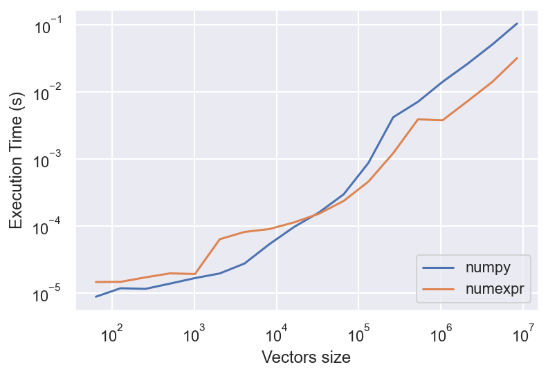
Fast Evaluation Of Array Expressions#
The
numexprpackage supplies routines for the fast evaluation of array expressions elementwise by using a vector-based virtual machine.Expressions are cached, so reuse is fast.
import numexpr as ne
import numpy as np
nrange = (2 ** np.arange(6, 24)).astype(int)

t_numpy = []
t_numexpr = []

for n in nrange:
    a = np.random.random(n)
    b = np.arange(n, dtype=np.double)
    c = np.random.random(n)

    c1 = ne.evaluate("a ** 2 + b ** 2 + 2 * a * b * c ", optimization='aggressive')

    t1 = %timeit -oq -n 10 a ** 2 + b ** 2 + 2 * a * b * c
    t2 = %timeit -oq -n 10 ne.re_evaluate()

    t_numpy.append(t1.best)
    t_numexpr.append(t2.best)

%matplotlib inline
%config InlineBackend.figure_format = 'retina'
import matplotlib.pyplot as plt
import seaborn; seaborn.set()

plt.loglog(nrange, t_numpy, label='numpy')
plt.loglog(nrange, t_numexpr, label='numexpr')

plt.legend(loc='lower right')
plt.xlabel('Vectors size')
plt.ylabel('Execution Time (s)');