Sympy

%matplotlib inline
%config InlineBackend.figure_format = "retina"
import matplotlib.pyplot as plt
import numpy as np
import seaborn as sns
sns.set()
plt.rcParams['figure.figsize'] = (10.0, 6.0)

The function init_printing() will enable LaTeX pretty printing in the notebook for SymPy expressions.

import sympy as sym
from sympy import symbols, Symbol
sym.init_printing()

x= Symbol('x')
(sym.pi + x)**2

alpha1, omega_2 = symbols('alpha1 omega_2')
alpha1, omega_2

mu, sigma = sym.symbols('mu sigma', positive = True)
1/sym.sqrt(2*sym.pi*sigma**2)* sym.exp(-(x-mu)**2/(2*sigma**2))

Why use sympy?

• Symbolic derivatives

• Translate mathematics into low level code

• Deal with very large expressions

• Optimize code using mathematics

Dividing two integers in Python creates a float, like 1/2 -> 0.5. If you want a rational number, use Rational(1, 2) or S(1)/2.

x + sym.S(1)/2 , sym.Rational(1,4)

y = Symbol('y')
x ^ y # XOR operator (True only if x != y)

x**y

SymPy expressions are immutable. Functions that operate on an expression return a new expression.

expr = x + 1
expr

expr.subs(x, 2)

expr

Exercise: Lagrange polynomial

Given a set of \(k + 1\) data points :\((x_0, y_0),\ldots,(x_j, y_j),\ldots,(x_k, y_k)\) the Lagrange interpolation polynomial is:

\[ L(x) := \sum_{j=0}^{k} y_j \ell_j(x) \]

\(\ell_j\) are Lagrange basis polynomials: $\(\ell_j(x) := \prod_{\begin{smallmatrix}0\le m\le k\\ m\neq j\end{smallmatrix}} \frac{x-x_m}{x_j-x_m} \)\( We can demonstrate that at each point \)x_i\(, \)L(x_i)=y_i\( so \)L$ interpolates the function.

• Compute the Lagrange polynomial for points $\( (-2,21),(-1,1),(0,-1),(1,-3),(2,1) \)$

Evaluate an expression

sym.sqrt(2), sym.sqrt(2).evalf(7) # set the precision to 7 digits

from sympy import sin
x = Symbol('x')
expr = sin(x)/x
expr.evalf(subs={x: 3.14})  # substitute the symbol x by Pi value

from sympy.utilities.autowrap import ufuncify
f = ufuncify([x], expr, backend='f2py') 

t = np.linspace(0,4*np.pi,100)
plt.plot(t, f(t));

---------------------------------------------------------------------------
TypeError                                 Traceback (most recent call last)
File /usr/share/miniconda3/envs/runenv/lib/python3.13/site-packages/sympy/core/cache.py:72, in __cacheit.<locals>.func_wrapper.<locals>.wrapper(*args, **kwargs)
     71 try:
---> 72     retval = cfunc(*args, **kwargs)
     73 except TypeError as e:

TypeError: unhashable type: 'list'

During handling of the above exception, another exception occurred:

TypeError                                 Traceback (most recent call last)
File /usr/share/miniconda3/envs/runenv/lib/python3.13/site-packages/sympy/core/cache.py:72, in __cacheit.<locals>.func_wrapper.<locals>.wrapper(*args, **kwargs)
     71 try:
---> 72     retval = cfunc(*args, **kwargs)
     73 except TypeError as e:

TypeError: unhashable type: 'list'

During handling of the above exception, another exception occurred:

CalledProcessError                        Traceback (most recent call last)
File /usr/share/miniconda3/envs/runenv/lib/python3.13/site-packages/sympy/utilities/autowrap.py:183, in CodeWrapper._process_files(self, routine)
    182 try:
--> 183     retoutput = check_output(command, stderr=STDOUT)
    184 except CalledProcessError as e:

File /usr/share/miniconda3/envs/runenv/lib/python3.13/subprocess.py:472, in check_output(timeout, *popenargs, **kwargs)
    470     kwargs['input'] = empty
--> 472 return run(*popenargs, stdout=PIPE, timeout=timeout, check=True,
    473            **kwargs).stdout

File /usr/share/miniconda3/envs/runenv/lib/python3.13/subprocess.py:577, in run(input, capture_output, timeout, check, *popenargs, **kwargs)
    576     if check and retcode:
--> 577         raise CalledProcessError(retcode, process.args,
    578                                  output=stdout, stderr=stderr)
    579 return CompletedProcess(process.args, retcode, stdout, stderr)

CalledProcessError: Command '['/usr/share/miniconda3/envs/runenv/bin/python', '-c', 'import numpy.f2py as f2py2e;f2py2e.main()', '-c', '-m', 'wrapper_module_0', 'wrapped_code_0.f90']' returned non-zero exit status 1.

During handling of the above exception, another exception occurred:

CodeWrapError                             Traceback (most recent call last)
Cell In[14], line 2
      1 from sympy.utilities.autowrap import ufuncify
----> 2 f = ufuncify([x], expr, backend='f2py') 
      4 t = np.linspace(0,4*np.pi,100)
      5 plt.plot(t, f(t));

File /usr/share/miniconda3/envs/runenv/lib/python3.13/site-packages/sympy/core/cache.py:76, in __cacheit.<locals>.func_wrapper.<locals>.wrapper(*args, **kwargs)
     74     if not e.args or not e.args[0].startswith('unhashable type:'):
     75         raise
---> 76     retval = func(*args, **kwargs)
     77 return retval

File /usr/share/miniconda3/envs/runenv/lib/python3.13/site-packages/sympy/utilities/autowrap.py:1177, in ufuncify(args, expr, language, backend, tempdir, flags, verbose, helpers, **kwargs)
   1175 args = [y] + indexed_args + [m]
   1176 args_with_indices = [a[i] for a in indexed_args]
-> 1177 return autowrap(Eq(y[i], f(*args_with_indices)), language, backend,
   1178                 tempdir, args, flags, verbose, helpers, **kwargs)

File /usr/share/miniconda3/envs/runenv/lib/python3.13/site-packages/sympy/core/cache.py:76, in __cacheit.<locals>.func_wrapper.<locals>.wrapper(*args, **kwargs)
     74     if not e.args or not e.args[0].startswith('unhashable type:'):
     75         raise
---> 76     retval = func(*args, **kwargs)
     77 return retval

File /usr/share/miniconda3/envs/runenv/lib/python3.13/site-packages/sympy/utilities/autowrap.py:690, in autowrap(expr, language, backend, tempdir, args, flags, verbose, helpers, code_gen, **kwargs)
    687         new_args.append(missing.name)
    688     routine = code_gen.routine('autofunc', expr, args + new_args)
--> 690 return code_wrapper.wrap_code(routine, helpers=helps)

File /usr/share/miniconda3/envs/runenv/lib/python3.13/site-packages/sympy/utilities/autowrap.py:164, in CodeWrapper.wrap_code(self, routine, helpers)
    162     self._generate_code(routine, helpers)
    163     self._prepare_files(routine)
--> 164     self._process_files(routine)
    165     mod = __import__(self.module_name)
    166 finally:

File /usr/share/miniconda3/envs/runenv/lib/python3.13/site-packages/sympy/utilities/autowrap.py:185, in CodeWrapper._process_files(self, routine)
    183     retoutput = check_output(command, stderr=STDOUT)
    184 except CalledProcessError as e:
--> 185     raise CodeWrapError(
    186         "Error while executing command: %s. Command output is:\n%s" % (
    187             " ".join(command), e.output.decode('utf-8')))
    188 if not self.quiet:
    189     print(retoutput)

CodeWrapError: Error while executing command: /usr/share/miniconda3/envs/runenv/bin/python -c import numpy.f2py as f2py2e;f2py2e.main() -c -m wrapper_module_0 wrapped_code_0.f90. Command output is:
Traceback (most recent call last):
  File "<string>", line 1, in <module>
    import numpy.f2py as f2py2e;f2py2e.main()
                                ~~~~~~~~~~~^^
  File "/usr/share/miniconda3/envs/runenv/lib/python3.13/site-packages/numpy/f2py/f2py2e.py", line 781, in main
    run_compile()
    ~~~~~~~~~~~^^
  File "/usr/share/miniconda3/envs/runenv/lib/python3.13/site-packages/numpy/f2py/f2py2e.py", line 753, in run_compile
    builder.compile()
    ~~~~~~~~~~~~~~~^^
  File "/usr/share/miniconda3/envs/runenv/lib/python3.13/site-packages/numpy/f2py/_backends/_meson.py", line 192, in compile
    self.run_meson(self.build_dir)
    ~~~~~~~~~~~~~~^^^^^^^^^^^^^^^^
  File "/usr/share/miniconda3/envs/runenv/lib/python3.13/site-packages/numpy/f2py/_backends/_meson.py", line 185, in run_meson
    self._run_subprocess_command(setup_command, build_dir)
    ~~~~~~~~~~~~~~~~~~~~~~~~~~~~^^^^^^^^^^^^^^^^^^^^^^^^^^
  File "/usr/share/miniconda3/envs/runenv/lib/python3.13/site-packages/numpy/f2py/_backends/_meson.py", line 181, in _run_subprocess_command
    subprocess.run(command, cwd=cwd, check=True)
    ~~~~~~~~~~~~~~^^^^^^^^^^^^^^^^^^^^^^^^^^^^^^
  File "/usr/share/miniconda3/envs/runenv/lib/python3.13/subprocess.py", line 554, in run
    with Popen(*popenargs, **kwargs) as process:
         ~~~~~^^^^^^^^^^^^^^^^^^^^^^
  File "/usr/share/miniconda3/envs/runenv/lib/python3.13/subprocess.py", line 1039, in __init__
    self._execute_child(args, executable, preexec_fn, close_fds,
    ~~~~~~~~~~~~~~~~~~~^^^^^^^^^^^^^^^^^^^^^^^^^^^^^^^^^^^^^^^^^
                        pass_fds, cwd, env,
                        ^^^^^^^^^^^^^^^^^^^
    ...<5 lines>...
                        gid, gids, uid, umask,
                        ^^^^^^^^^^^^^^^^^^^^^^
                        start_new_session, process_group)
                        ^^^^^^^^^^^^^^^^^^^^^^^^^^^^^^^^^
  File "/usr/share/miniconda3/envs/runenv/lib/python3.13/subprocess.py", line 1972, in _execute_child
    raise child_exception_type(errno_num, err_msg, err_filename)
FileNotFoundError: [Errno 2] No such file or directory: 'meson'
Cannot use distutils backend with Python>=3.12, using meson backend instead.
Using meson backend
Will pass --lower to f2py
See https://numpy.org/doc/stable/f2py/buildtools/meson.html
Reading fortran codes...
	Reading file 'wrapped_code_0.f90' (format:free)
Post-processing...
	Block: wrapper_module_0
			Block: autofunc
Applying post-processing hooks...
  character_backward_compatibility_hook
Post-processing (stage 2)...
Building modules...
    Building module "wrapper_module_0"...
    Generating possibly empty wrappers"
    Maybe empty "wrapper_module_0-f2pywrappers.f"
        Constructing wrapper function "autofunc"...
          y_3625019 = autofunc(x_3625023,[m_3625020])
    Wrote C/API module "wrapper_module_0" to file "./wrapper_module_0module.c"

Exercise

• Plot the Lagrange polynomial computed above and interpolations points with matplotlib

Undefined functions and derivatives

Undefined functions are created with Function(). Undefined are useful to state that one variable depends on another (for the purposes of differentiation).

from sympy import Function
f = Function('f')

f(x) + 1

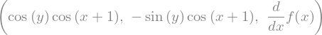
from sympy import diff, sin, cos
diff(sin(x + 1)*cos(y), x), diff(sin(x + 1)*cos(y), x, y), diff(f(x), x)

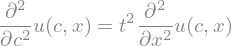
c, t = sym.symbols('t c')
u = sym.Function('u')
sym.Eq(diff(u(t,x),t,t), c**2*diff(u(t,x),x,2))

Matrices

from sympy import Matrix
Matrix([[1, 2], [3, 4]])*Matrix([x, y])

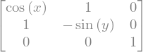
x, y, z = sym.symbols('x y z')
Matrix([sin(x) + y, cos(y) + x, z]).jacobian([x, y, z])

Matrix symbols

SymPy can also operate on matrices of symbolic dimension (\(n \times m\)). MatrixSymbol("M", n, m) creates a matrix \(M\) of shape \(n \times m\).

from sympy import MatrixSymbol, Transpose

n, m = sym.symbols('n m', integer=True)
M = MatrixSymbol("M", n, m)
b = MatrixSymbol("b", m, 1)
Transpose(M*b)

Transpose(M*b).doit()

Solving systems of equations

solve solves equations symbolically (not numerically). The return value is a list of solutions. It automatically assumes that it is equal to 0.

from sympy import Eq, solve
solve(Eq(x**2, 4), x)

solve(x**2 + 3*x - 3, x)

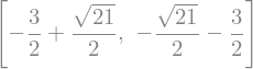
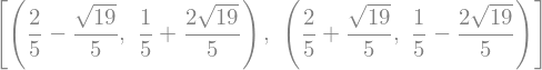
eq1 = x**2 + y**2 - 4  # circle of radius 2
eq2 = 2*x + y - 1  # straight line: y(x) = -2*x + 1
solve([eq1, eq2], [x, y])

Solving differential equations

dsolve can (sometimes) produce an exact symbolic solution. Like solve, dsolve assumes that expressions are equal to 0.

from sympy import Function, dsolve
f = Function('f')
dsolve(f(x).diff(x, 2) + f(x))

Code printers

The most basic form of code generation are the code printers. They convert SymPy expressions into over a dozen target languages.

x = symbols('x')
expr = abs(sin(x**2))
expr

sym.ccode(expr)

'fabs(sin(pow(x, 2)))'

sym.fcode(expr, standard=2003, source_format='free')

'abs(sin(x**2))'

from sympy.printing.cxxcode import cxxcode
cxxcode(expr)

'std::fabs(std::sin(std::pow(x, 2)))'

sym.tanh(x).rewrite(sym.exp)

from sympy import sqrt, exp, pi
expr = 1/sqrt(2*pi*sigma**2)* exp(-(x-mu)**2/(2*sigma**2))
print(sym.fcode(expr, standard=2003, source_format='free'))

parameter (pi = 3.1415926535897932d0)
(1.0d0/2.0d0)*sqrt(2.0d0)*exp(-0.5d0*(-mu + x)**2/sigma**2)/(sqrt(pi)* &
      sigma)

Creating a function from a symbolic expression

In SymPy there is a function to create a Python function which evaluates (usually numerically) an expression. SymPy allows the user to define the signature of this function (which is convenient when working with e.g. a numerical solver in scipy).

from sympy import log
x, y = symbols('x y')
expr = 3*x**2 + log(x**2 + y**2 + 1)
expr

%timeit expr.subs({x: 17, y: 42}).evalf()

478 µs ± 50.7 µs per loop (mean ± std. dev. of 7 runs, 1000 loops each)

import math
f = lambda x, y: 3*x**2 + math.log(x**2 + y**2 + 1)
f(17, 42)

%timeit f(17, 42)

3.84 µs ± 614 ns per loop (mean ± std. dev. of 7 runs, 100000 loops each)

Evaluate above expression numerically invoking the subs method followed by the evalf method can be quite slow and cannot be done repeatedly.

from sympy import lambdify
g = lambdify([x, y], expr, modules=['math'])
g(17, 42)

%timeit g(17, 42)

3.67 µs ± 715 ns per loop (mean ± std. dev. of 7 runs, 100000 loops each)

xarr = np.linspace(17, 18, 5)
h = lambdify([x, y], expr)  # lambdify return a python function
out = h(xarr, 42)
out.shape

z = z1, z2, z3 = symbols('z:3')
expr2 = x*y*(z1 + z2 + z3)
func2 = lambdify([x, y, z], expr2)
func2(1, 2, (3, 4, 5))

Behind the scenes lambdify constructs a string representation of the Python code and uses Python’s eval function to compile the function.

SIR model

\begin{align} \frac{dS(t)}{dt} &= - \beta S(t) I(t) \ \frac{dI(t)}{dt} &= \beta S(t) I(t) - \gamma I(t) \ \frac{dR(t)}{dt} &= \gamma I(t) \end{align}

• S,I,R: ratio of suceptibles, infectious and recovered fraction of the population.

• t: time

• \(\beta\) : transmission coefficient.

• \(\gamma\) : healing rate.

We assume that total population is constant.

Solving the initial value problem numerically

We will now integrate this system of ordinary differential equations numerically using the odeint solver provided by scipy:

By looking at the documentation of odeint we see that we need to provide a function which computes a vector of derivatives (\(\dot{\mathbf{y}} = [\frac{dy_1}{dt}, \frac{dy_2}{dt}, \frac{dy_3}{dt}]\)). The expected signature of this function is:

f(y: array[float64], t: float64, *args: arbitrary constants) -> dydt: array[float64]

in our case we can write it as:

def rhs(y, t, beta, gamma):
    rb = beta * y[0]*y[1]
    rg = gamma * y[1]
    return [- rb , rb - rg, rg]

import scipy.integrate as spi
tout = np.linspace(0, 10, 100)
k_vals = 1.66, 0.4545455
y0 = [0.95, 0.05, 0]
yout = spi.odeint(rhs, y0, tout, k_vals)
plt.plot(tout, yout)
plt.legend(['susceptible', 'infected', 'recovered']);

We will construct the system from a symbolic representation. But at the same time, we need the rhs function to be fast. Which means that we want to produce a fast function from our symbolic representation. Generating a function from our symbolic representation is achieved through code generation.

1. Construct a symbolic representation from some domain specific representation using SymPy.

2. Have SymPy generate a function with an appropriate signature (or multiple thereof), which we pass on to the solver.

We will achieve (1) by using SymPy symbols (and functions if needed). For (2) we will use a function in SymPy called lambdify―it takes a symbolic expressions and returns a function. In a later notebook, we will look at (1), for now we will just use rhs which we’ve already written:

y, k = sym.symbols('y:3'), sym.symbols('beta gamma')
ydot = rhs(y, None, *k)
y, ydot

f = sym.lambdify((y,t)+k, ydot)
plt.plot(tout, spi.odeint(f, y0, tout, k_vals))
plt.legend(['Suceptible', 'Infected', 'Recovered']);

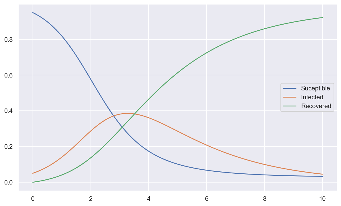
In this example the gains of using a symbolic representation are arguably limited.

Let’s take the same example with demography and \(n\) classes of subjects:

\[ X_i = S_i, I_i, R_i \qquad i = 1 \ldots n \]

\[\begin{split} \frac{dS_i}{dt} = \nu_i - \beta_i S_i I_i - \mu_i S_i + \sum_{j=1}^n m_{ji} S_j-\sum_{j=1}^n m_{ij} S_i \\ \frac{dI_i}{dt} = \beta_i S_i I_i - (\gamma_i + \mu_i) I_i + \sum_{j=1}^n m_{ij} I_j-\sum_{j=1}^n m_{ji} I_i \\ \frac{dR_i}{dt} = - \frac{dS_i}{dt} - \frac{dI_i}{dt} \end{split}\]

• \(\beta\) : transmission coefficient

• \(\gamma\) : healing rate

• \(\mu\) : mortality rate

• \(\nu\) : birth rate

Exercise

• Create the symbolic matrix \(m\), symbols \(\nu_i,\mu_i,\beta_i,\gamma_i\) for \(i=0,1,2\) and \(y_j\) for \(j=0,1,2,\ldots,8\)

• Write the system \(\dot{y} = f(t,y,m,\nu,\mu,\beta,\gamma)\)

• lambdify the \(f\) function.

• Solve the system with: $\( m = \begin{bmatrix} 0 & 0.01 & 0.01 \\ 0.01 & 0 & 0.01 \\ 0.01 & 0.01 & 0 \\ \end{bmatrix} \)\( \)\( \begin{aligned} t &= [0,10] \mbox{ with } dt = 0.1 \\ \nu_i &= 0.0 \\ \mu_i &= 0.0 \\ \beta_i &= 1.66 \\ \gamma_i &= [0.4545,0.3545,0.2545] \\ S_i&= 0.95 \\ I_i &= 0.05 \\ R_i &= 0.0 \end{aligned} \)$

Exercise : Bezier curve

We want to compute and the draw the Bezier curve between the 3 points \(p_0\), \(p_1\), and \(p_2\), The middle point \(p_1\) position is arbitrary.

\[ p0=(1,0); \qquad p1=(x,y); \qquad p2=(0,1) \]

The \(n+1\) Bernstein basis polynomials of degree \(n\) are defined as

\[ b_{i,n}(x) = {n \choose i} x^{i} \left( 1 - x \right)^{n - i}, \quad i = 0, \ldots, n. \]

where \({n \choose i}\) is the binomial coefficient.

The Bezier curve is defined by a linear combination of Bernstein basis polynomials:

\[B_n(x) = \sum_{i=0}^{n} \beta_{i} b_{i,n}(x)\]

• Withsympy.binomial, write a function bpoly(t,n,i) that returns the Bernstein basis polynomial \(b_{i,n}(t)\).

• Compute the Berstein polynomial representing the Bezier curve between \(p_0,p_1,p_2\). \(\beta_i=1\).

• Plot the Bezier Curve for 3 positions of \(p_1= (0,0), (0.5,0.5), (1,1)\)

Integrals quadrature

from sympy.integrals.quadrature import *
x, w = gauss_legendre(3, 5)
x, w

x, w = gauss_lobatto(3,12)
x, w

References

• SciPy 2017 tutorial