Scipy#

scipy

Scipy is the scientific Python ecosystem :

fft, linear algebra, scientific computation,…
scipy contains numpy, it can be considered as an extension of numpy.
the add-on toolkits Scikits complements scipy.

%matplotlib inline
%config InlineBackend.figure_format = 'retina'
import numpy as np
import scipy as sp
import matplotlib.pyplot as plt
plt.rcParams['figure.figsize'] = (10,6)

SciPy main packages#

constants : Physical and mathematical constants
fftpack : Fast Fourier Transform routines
integrate : Integration and ordinary differential equation solvers
interpolate : Interpolation and smoothing splines
io : Input and Output
linalg : Linear algebra
signal : Signal processing
sparse : Sparse matrices and associated routines

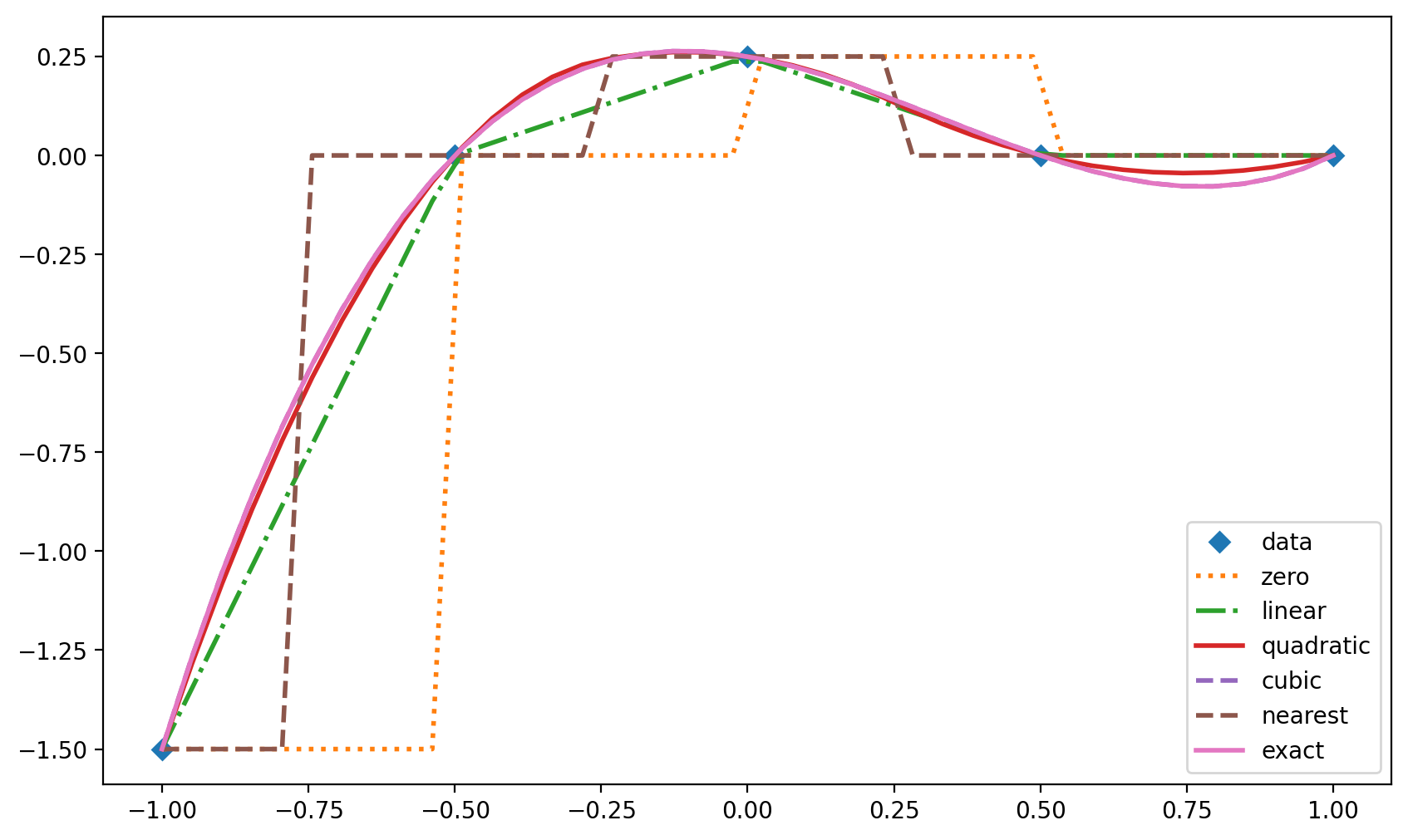
from scipy.interpolate import interp1d 
x = np.linspace(-1, 1, num=5)  # 5 points evenly spaced in [-1,1].
y = (x-1.)*(x-0.5)*(x+0.5)     # x and y are numpy arrays
f0 = interp1d(x,y, kind='zero')
f1 = interp1d(x,y, kind='linear') 
f2 = interp1d(x,y, kind='quadratic') 
f3 = interp1d(x,y, kind='cubic') 
f4 = interp1d(x,y, kind='nearest') 

xnew = np.linspace(-1, 1, num=40) 
ynew = (xnew-1.)*(xnew-0.5)*(xnew+0.5) 
plt.plot(x,y,'D',xnew,f0(xnew),':', xnew, f1(xnew),'-.',
                xnew,f2(xnew),'-',xnew ,f3(xnew),'--',
                xnew,f4(xnew),'--',xnew, ynew, linewidth=2)
plt.legend(['data','zero','linear','quadratic','cubic','nearest','exact'],
          loc='best');

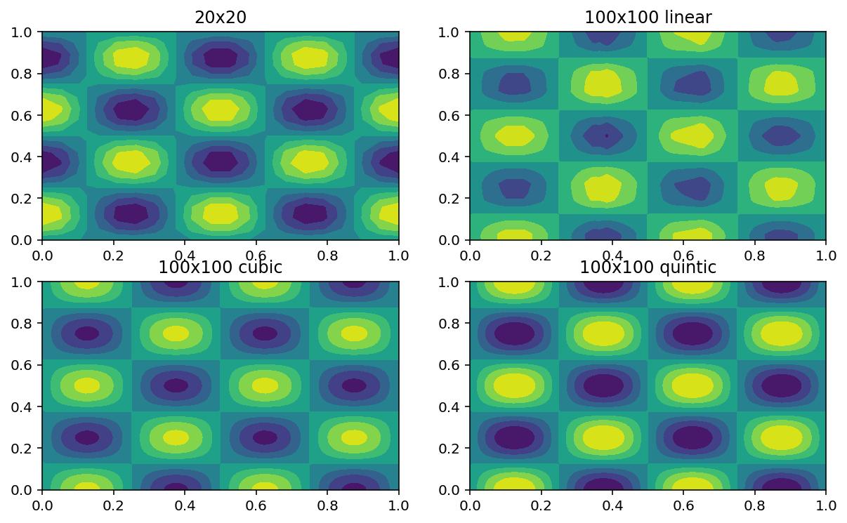
from scipy.interpolate import interp2d
x,y = sp.mgrid[0:1:20j,0:1:20j]  #create the grid 20x20
z = np.cos(4*sp.pi*x)*np.sin(4*sp.pi*y) #initialize the field
T1=interp2d(x,y,z,kind='linear') 
T2=interp2d(x,y,z,kind='cubic') 
T3=interp2d(x,y,z,kind='quintic')

/tmp/ipykernel_11140/3016852277.py:4: DeprecationWarning: `interp2d` is deprecated!
`interp2d` is deprecated in SciPy 1.10 and will be removed in SciPy 1.12.0.

For legacy code, nearly bug-for-bug compatible replacements are
`RectBivariateSpline` on regular grids, and `bisplrep`/`bisplev` for
scattered 2D data.

In new code, for regular grids use `RegularGridInterpolator` instead.
For scattered data, prefer `LinearNDInterpolator` or
`CloughTocher2DInterpolator`.

For more details see
`https://gist.github.com/ev-br/8544371b40f414b7eaf3fe6217209bff`

  T1=interp2d(x,y,z,kind='linear')
/tmp/ipykernel_11140/3016852277.py:5: DeprecationWarning: `interp2d` is deprecated!
`interp2d` is deprecated in SciPy 1.10 and will be removed in SciPy 1.12.0.

For legacy code, nearly bug-for-bug compatible replacements are
`RectBivariateSpline` on regular grids, and `bisplrep`/`bisplev` for
scattered 2D data.

In new code, for regular grids use `RegularGridInterpolator` instead.
For scattered data, prefer `LinearNDInterpolator` or
`CloughTocher2DInterpolator`.

For more details see
`https://gist.github.com/ev-br/8544371b40f414b7eaf3fe6217209bff`

  T2=interp2d(x,y,z,kind='cubic')
/tmp/ipykernel_11140/3016852277.py:6: DeprecationWarning: `interp2d` is deprecated!
`interp2d` is deprecated in SciPy 1.10 and will be removed in SciPy 1.12.0.

For legacy code, nearly bug-for-bug compatible replacements are
`RectBivariateSpline` on regular grids, and `bisplrep`/`bisplev` for
scattered 2D data.

In new code, for regular grids use `RegularGridInterpolator` instead.
For scattered data, prefer `LinearNDInterpolator` or
`CloughTocher2DInterpolator`.

For more details see
`https://gist.github.com/ev-br/8544371b40f414b7eaf3fe6217209bff`

  T3=interp2d(x,y,z,kind='quintic')

X,Y=sp.mgrid[0:1:100j,0:1:100j] #create the interpolation grid 100x100 
# complex -> number of points, float -> step size
plt.figure(1) 
plt.subplot(221) #Plot original data
plt.contourf(x,y,z) 
plt.title('20x20') 
plt.subplot(222) #Plot linear interpolation
plt.contourf(X,Y,T1(X[:,0],Y[0,:])) 
plt.title('100x100 linear') 
plt.subplot(223) #Plot cubic interpolation
plt.contourf(X,Y,T2(X[:,0],Y[0,:])) 
plt.title('100x100 cubic')
plt.subplot(224) #Plot quintic interpolation
plt.contourf(X,Y,T3(X[:,0],Y[0,:])) 
plt.title('100x100 quintic') 

/tmp/ipykernel_11140/2191985395.py:8: DeprecationWarning:         `interp2d` is deprecated!
        `interp2d` is deprecated in SciPy 1.10 and will be removed in SciPy 1.12.0.

        For legacy code, nearly bug-for-bug compatible replacements are
        `RectBivariateSpline` on regular grids, and `bisplrep`/`bisplev` for
        scattered 2D data.

        In new code, for regular grids use `RegularGridInterpolator` instead.
        For scattered data, prefer `LinearNDInterpolator` or
        `CloughTocher2DInterpolator`.

        For more details see
        `https://gist.github.com/ev-br/8544371b40f414b7eaf3fe6217209bff`

  plt.contourf(X,Y,T1(X[:,0],Y[0,:]))
/tmp/ipykernel_11140/2191985395.py:11: DeprecationWarning:         `interp2d` is deprecated!
        `interp2d` is deprecated in SciPy 1.10 and will be removed in SciPy 1.12.0.

        For legacy code, nearly bug-for-bug compatible replacements are
        `RectBivariateSpline` on regular grids, and `bisplrep`/`bisplev` for
        scattered 2D data.

        In new code, for regular grids use `RegularGridInterpolator` instead.
        For scattered data, prefer `LinearNDInterpolator` or
        `CloughTocher2DInterpolator`.

        For more details see
        `https://gist.github.com/ev-br/8544371b40f414b7eaf3fe6217209bff`

  plt.contourf(X,Y,T2(X[:,0],Y[0,:]))
/tmp/ipykernel_11140/2191985395.py:14: DeprecationWarning:         `interp2d` is deprecated!
        `interp2d` is deprecated in SciPy 1.10 and will be removed in SciPy 1.12.0.

        For legacy code, nearly bug-for-bug compatible replacements are
        `RectBivariateSpline` on regular grids, and `bisplrep`/`bisplev` for
        scattered 2D data.

        In new code, for regular grids use `RegularGridInterpolator` instead.
        For scattered data, prefer `LinearNDInterpolator` or
        `CloughTocher2DInterpolator`.

        For more details see
        `https://gist.github.com/ev-br/8544371b40f414b7eaf3fe6217209bff`

  plt.contourf(X,Y,T3(X[:,0],Y[0,:]))

Text(0.5, 1.0, '100x100 quintic')

FFT : scipy.fftpack#

FFT dimension 1, 2 and n : fft, ifft (inverse), rfft (real), irfft, fft2 (dimension 2), ifft2, fftn (dimension n), ifftn.
Discrete cosinus transform : dct
Convolution product : convolve

from numpy.fft import fft, ifft
x = np.random.random(2048)
%timeit ifft(fft(x))

47.1 µs ± 28.7 ns per loop (mean ± std. dev. of 7 runs, 10,000 loops each)

from scipy.fftpack import fft, ifft
x = np.random.random(2048)
%timeit ifft(fft(x))

45.8 µs ± 55.9 ns per loop (mean ± std. dev. of 7 runs, 10,000 loops each)

Linear algebra : scipy.linalg#

Sovers, decompositions, eigen values. (same as numpy).
Matrix functions : expm, sinm, sinhm,…
Block matrices diagonal, triangular, periodic,…

import scipy.linalg as spl 
b=np.ones(5)
A=np.array([[1.,3.,0., 0.,0.],
           [ 2.,1.,-4, 0.,0.],
           [ 6.,1., 2,-3.,0.], 
           [ 0.,1., 4.,-2.,-3.], 
           [ 0.,0., 6.,-3., 2.]])
print("x=",spl.solve(A,b,sym_pos=False)) # LAPACK ( gesv ou posv )
AB=np.array([[0.,3.,-4.,-3.,-3.],
             [1.,1., 2.,-2., 2.],
             [2.,1., 4.,-3., 0.],
             [6.,1., 6., 0., 0.]])
print("x=",spl.solve_banded((2,1),AB,b)) # LAPACK ( gbsv )

x= [-0.24074074  0.41358025 -0.26697531 -0.85493827  0.01851852]
x= [-0.24074074  0.41358025 -0.26697531 -0.85493827  0.01851852]

P,L,U = spl.lu(A) #  P A = L U
np.set_printoptions(precision=3)
for M in (P,L,U):
    print(M, end="\n"+20*"-"+"\n")

[[0. 1. 0. 0. 0.]
 [0. 0. 0. 1. 0.]
 [1. 0. 0. 0. 0.]
 [0. 0. 0. 0. 1.]
 [0. 0. 1. 0. 0.]]
--------------------
[[ 1.     0.     0.     0.     0.   ]
 [ 0.167  1.     0.     0.     0.   ]
 [ 0.     0.     1.     0.     0.   ]
 [ 0.333  0.235 -0.765  1.     0.   ]
 [ 0.     0.353  0.686  0.083  1.   ]]
--------------------
[[ 6.     1.     2.    -3.     0.   ]
 [ 0.     2.833 -0.333  0.5    0.   ]
 [ 0.     0.     6.    -3.     2.   ]
 [ 0.     0.     0.    -1.412  1.529]
 [ 0.     0.     0.     0.    -4.5  ]]
--------------------

CSC (Compressed Sparse Column)#

All operations are optimized
Efficient “slicing” along axis=1.
Fast Matrix-vector product.
Conversion to other format could be costly.

import scipy.sparse as spsp
row = np.array([0,2,2,0,1,2]) 
col = np.array([0,0,1,2,2,2])
data  = np.array([1,2,3,4,5,6]) 
Mcsc1 = spsp.csc_matrix((data,(row,col)),shape=(3,3)) 
Mcsc1.todense()

matrix([[1, 0, 4],
        [0, 0, 5],
        [2, 3, 6]])

indptr  = np.array([0,2,3,6]) 
indices = np.array([0,2,2,0,1,2]) 
data    = np.array([1,2,3,4,5,6]) 
Mcsc2 = spsp.csc_matrix ((data,indices,indptr),shape=(3,3))
Mcsc2.todense()

matrix([[1, 0, 4],
        [0, 0, 5],
        [2, 3, 6]])

Dedicated format for assembling#

lil_matrix : Row-based linked list matrix. Easy format to build your matrix and convert to other format before solving.
dok_matrix : A dictionary of keys based matrix. Ideal format for incremental matrix building. The conversion to csc/csr format is efficient.
coo_matrix : coordinate list format. Fast conversion to formats CSC/CSR.

Lien vers la documentation scipy

Sparse matrices : scipy.sparse.linalg #

speigen, speigen_symmetric, lobpcg : (ARPACK).
svd : (ARPACK).
Direct methods (UMFPACK or SUPERLU) or Krylov based methods
Minimization : lsqr and minres

For linear algebra:

Noobs: spsolve.
Intermmediate: dsolve.spsolve or isolve.spsolve
Advanced: splu, spilu (direct); cg, cgs, bicg, bicgstab, gmres, lgmres et qmr (iterative)
Boss: petsc4py et slepc4py.

LinearOperator#

The LinearOperator is used for matrix-free numerical methods.

import scipy.sparse.linalg as spspl
def mv(v):
   return np.array([2*v[0],3*v[1]])

A=spspl.LinearOperator((2 ,2),matvec=mv,dtype=float )
A

<2x2 _CustomLinearOperator with dtype=float64>

A*np.ones(2)

array([2., 3.])

A.matmat(np.array([[1,-2],[3,6]]))

array([[ 2, -4],
       [ 9, 18]])

LU decomposition#

N = 50
un = np.ones(N)
w = np.random.rand(N+1)
A = spsp.spdiags([w[1:],-2*un,w[:-1]],[-1,0,1],N,N) # tridiagonal matrix
A = A.tocsc()
b = un
op = spspl.splu(A)
op

<SuperLU at 0x7f7f0068a160>

x=op.solve(b)
spl.norm(A*x-b)

1.456043846448818e-15

Conjugate Gradient#

global k
k=0
def f(xk): # function called at every iterations
     global k
     print ("iteration {0:2d} residu = {1:7.3g}".format(k,spl.norm(A*xk-b)))
     k += 1

x,info=spspl.cg(A,b,x0=np.zeros(N),tol=1.0e-12,maxiter=N,M=None,callback=f)

iteration  0 residu =    2.54
iteration  1 residu =   0.925
iteration  2 residu =   0.431
iteration  3 residu =   0.157
iteration  4 residu =  0.0666
iteration  5 residu =  0.0241
iteration  6 residu = 0.00982
iteration  7 residu = 0.00392
iteration  8 residu = 0.00132
iteration  9 residu = 0.000454
iteration 10 residu = 0.000173
iteration 11 residu = 6.04e-05
iteration 12 residu = 2.05e-05
iteration 13 residu = 6.08e-06
iteration 14 residu = 2.06e-06
iteration 15 residu = 6.83e-07
iteration 16 residu = 2.59e-07
iteration 17 residu = 8.2e-08
iteration 18 residu = 3.47e-08
iteration 19 residu = 1.01e-08
iteration 20 residu = 3.21e-09
iteration 21 residu = 9.91e-10
iteration 22 residu = 3.21e-10
iteration 23 residu = 1.03e-10
iteration 24 residu = 3.77e-11
iteration 25 residu = 1.16e-11
iteration 26 residu = 3.12e-12

Preconditioned conjugate gradient#

pc=spspl.spilu(A,drop_tol=0.1)  # pc is an ILU decomposition
xp=pc.solve(b)
spl.norm(A*xp-b)

0.29015179575537214

def mv(v):
    return pc.solve(v)
lo = spspl.LinearOperator((N,N),matvec=mv)
k = 0
x,info=spspl.cg(A,b,x0=np.zeros(N),tol=1.e-12,maxiter=N,M=lo,callback=f)

iteration  0 residu =   0.272
iteration  1 residu =  0.0124
iteration  2 residu = 0.00073
iteration  3 residu = 2.51e-05
iteration  4 residu = 9.88e-07
iteration  5 residu = 4.47e-08
iteration  6 residu = 3.29e-09
iteration  7 residu = 1.42e-10
iteration  8 residu = 1.04e-11
iteration  9 residu = 6.41e-13

Numerical integration#

quad, dblquad, tplquad,… Fortran library QUADPACK.

import scipy.integrate as spi

x2=lambda x: x**2
4.**3/3  # int(x2) in [0,4]

21.333333333333332

spi.quad(x2,0.,4.)

(21.333333333333336, 2.368475785867001e-13)

Scipy ODE solver#

It uses the Fortran ODEPACK library.

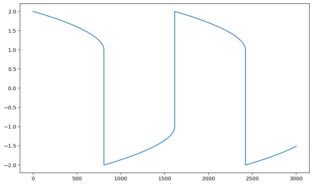
Van der Pol Oscillator#

\begin{align} y_1’(t) & = y_2(t), \nonumber \ y_2’(t) & = 1000(1 - y_1^2(t))y_2(t) - y_1(t) \nonumber \end{align} $$ with $y_1(0) = 2 $ and $ y_2(0) = 0. $.

import numpy as np
import scipy.integrate as spi

def vdp1000(y,t):
     dy=np.zeros(2)
     dy[0]=y[1]
     dy[1]=1000.*(1.-y[0]**2)*y[1]-y[0]
     return dy 

t0, tf =0,  3000
N = 300000
t, dt = np.linspace(t0,tf,N, retstep=True)

y=spi.odeint(vdp1000,[2.,0.],t)
plt.plot(t,y[:,0]);

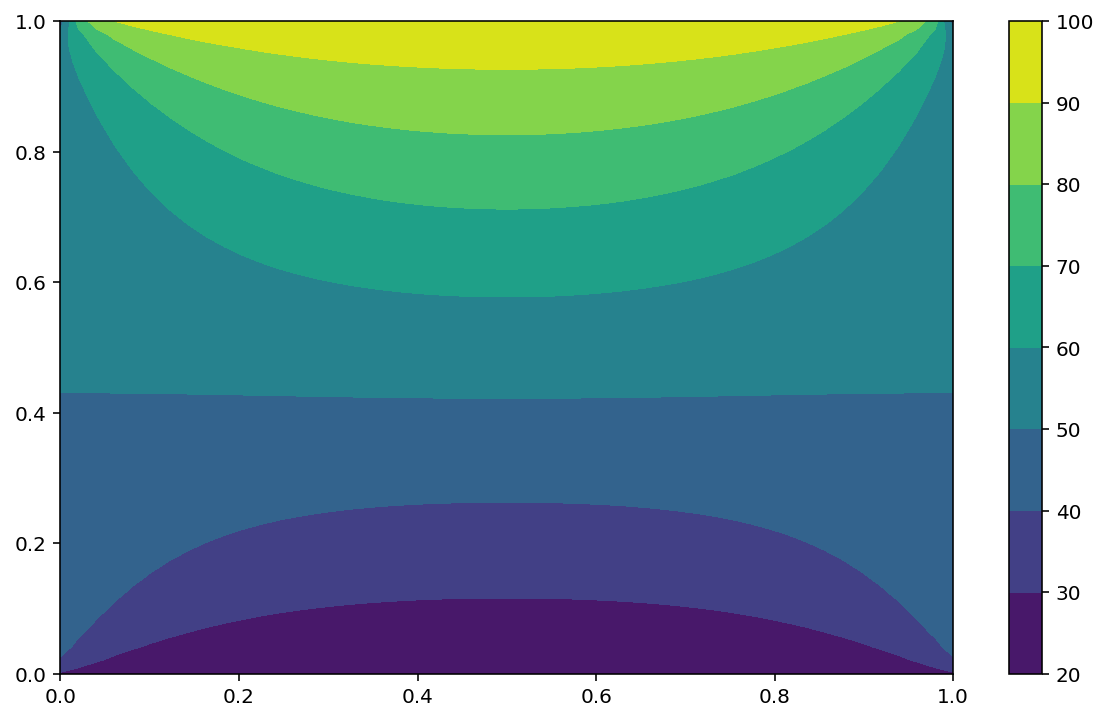
Exercise#

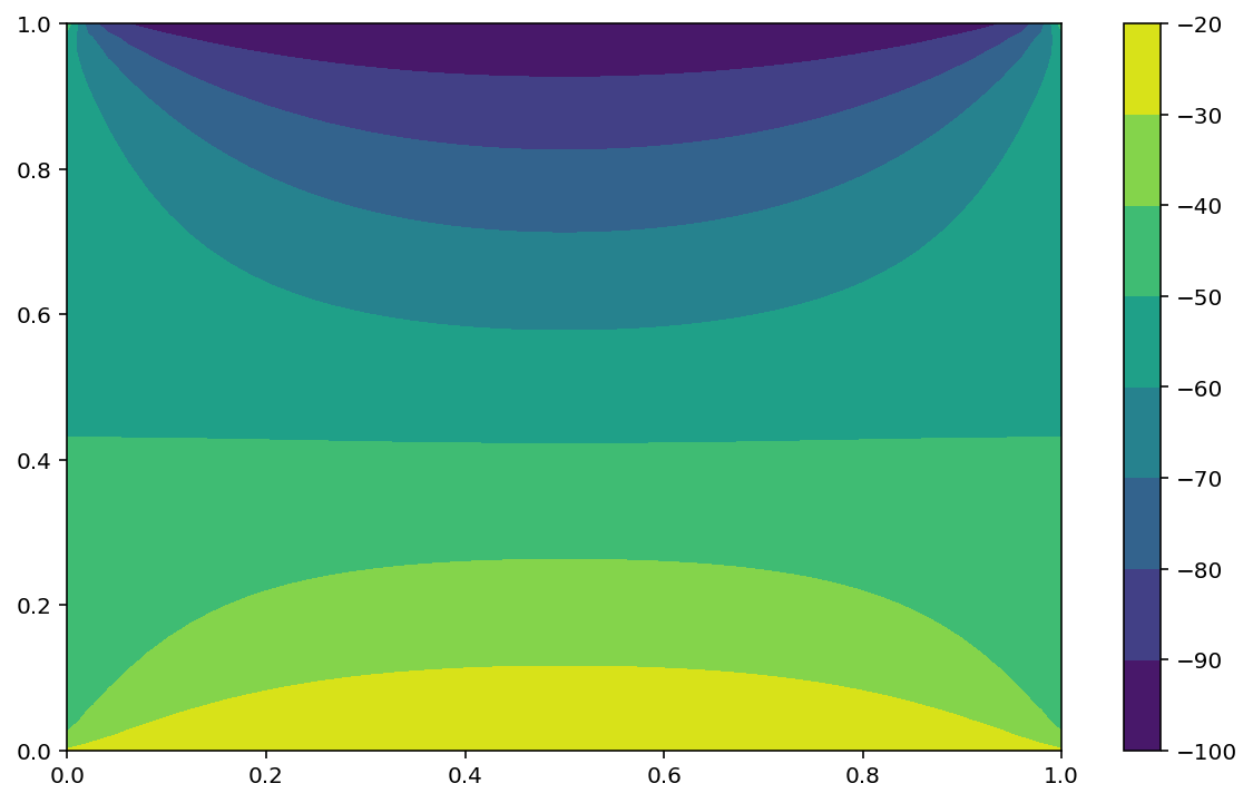
The following code solve the Laplace equation using a dense matrix.

Modified the code to use a sparse matrix

%matplotlib inline
%config InlineBackend.figure_format = "retina"
import numpy as np
import matplotlib.pyplot as plt
plt.rcParams['figure.figsize'] = (10,6)

# Boundary conditions
Tnorth, Tsouth, Twest, Teast = 100, 20, 50, 50

# Set meshgrid
n = 50
l = 1.0
h = l / (n-1)
X, Y = np.meshgrid(np.linspace(0,l,n), np.linspace(0,l,n))
T = np.zeros((n,n),dtype='d')

# Set Boundary condition
T[n-1:, :] = Tnorth / h**2
T[:1, :] = Tsouth / h**2
T[:, n-1:] = Teast / h**2
T[:, :1] = Twest / h**2

A = np.zeros((n*n,n*n),dtype='d')
nn = n*n
ii = 0
for j in range(n):
    for i in range(n):   
      if j > 0:
         jj = ii - n
         A[ii,jj] = -1
      if j < n-1: 
         jj = ii + n
         A[ii,jj] = -1
      if i > 0:
         jj = ii - 1
         A[ii,jj] = -1
      if i < n-1:
         jj = ii + 1
         A[ii,jj] = -1
      A[ii,ii] = 4
      ii = ii+1

%%time
U = np.linalg.solve(A,np.ravel(h**2*T))

CPU times: user 210 ms, sys: 40.1 ms, total: 250 ms
Wall time: 140 ms

T = U.reshape(n,n)
plt.contourf(X,Y,T)
plt.colorbar()

<matplotlib.colorbar.Colorbar at 0x7f7f0019c370>

import scipy.sparse as spsp
import scipy.sparse.linalg as spspl

# Boundary conditions
Tnorth, Tsouth, Twest, Teast = 100, 20, 50, 50

# Set meshgrid
n = 50
l = 1.0
h = l / (n-1)
X, Y = np.meshgrid(np.linspace(0,l,n), np.linspace(0,l,n))
T = np.zeros((n,n),dtype='d')

# Set Boundary condition
T[n-1:, :]    = Tnorth / h**2
T[  :1, :]    = Tsouth / h**2
T[   :, n-1:] = Teast  / h**2
T[   :, :1]   = Twest  / h**2

bdiag = -4 * np.eye(n)
bup   = np.diag([1] * (n - 1), 1)
blow  = np.diag([1] * (n - 1), -1)
block = bdiag + bup + blow
# Creat a list of n blocks
blist = [block] * n
S = spsp.block_diag(blist)
# Upper diagonal array offset by -n
upper = np.diag(np.ones(n * (n - 1)), n)
# Lower diagonal array offset by -n
lower = np.diag(np.ones(n * (n - 1)), -n)
S += upper + lower

%%time
U = sp.linalg.solve(S,np.ravel(h**2*T))

CPU times: user 395 ms, sys: 32 ms, total: 427 ms
Wall time: 289 ms

plt.contourf(X,Y,U.reshape(n,n))
plt.colorbar();

Python notebooks

Scipy

Contents

Scipy#

SciPy main packages#

FFT : scipy.fftpack#

Linear algebra : scipy.linalg#

CSC (Compressed Sparse Column)#

Dedicated format for assembling#

Sparse matrices : scipy.sparse.linalg #

LinearOperator#

LU decomposition#

Conjugate Gradient#

Preconditioned conjugate gradient#

Numerical integration#

Scipy ODE solver#

Van der Pol Oscillator#

Exercise#

Python notebooks

Scipy

Contents

Scipy#

SciPy main packages#

FFT : scipy.fftpack#

Linear algebra : scipy.linalg#

CSC (Compressed Sparse Column)#

Dedicated format for assembling#

Sparse matrices : scipy.sparse.linalg#

LinearOperator#

LU decomposition#

Conjugate Gradient#

Preconditioned conjugate gradient#

Numerical integration#

Scipy ODE solver#

Van der Pol Oscillator#

Exercise#

Sparse matrices : scipy.sparse.linalg #